---
title: "Part 2: Spatial & Statistical Analysis"
subtitle: "Understanding Distribution Patterns and Grade Characteristics"
author: "Ghozian Islam Karami"
date: "2025-10-03"
categories: [EDA, Spatial Analysis, Statistics, Visualization]
image: "Part2.png"
format:
html:
code-fold: true
code-tools: true
toc: true
toc-depth: 3
---
## Introduction
With validated data from [Part 1](/posts/Data Validation/), we now explore **where** the data is located and **what** it tells us statistically. This post covers:
- **Pillar 2**: Spatial Distribution Analysis
- **Pillar 3**: Statistical Characterization
These pillars help us understand sampling density, identify spatial patterns, and characterize grade distributions - all critical for informed estimation decisions.
## Setup and Data Loading
```{r}
#| message: false
#| warning: false
library(dplyr)
library(tidyr)
library(ggplot2)
library(plotly)
library(DT)
library(RColorBrewer)
library(patchwork)

# Create simulated drilling data
set.seed(123)
n_holes <- 50

collar <- data.frame(
  hole_id = paste0("DDH", sprintf("%03d", 1:n_holes)),
  x = runif(n_holes, 500000, 501000),
  y = runif(n_holes, 9000000, 9001000),
  rl = runif(n_holes, 100, 200)
)

# Assay data with spatial correlation
assay_list <- lapply(1:n_holes, function(i) {
  n_intervals <- sample(15:25, 1)
  depths <- seq(0, by = 2, length.out = n_intervals)

  # Add spatial correlation to grades
  distance_from_center <- sqrt((collar$x[i] - 500500)^2 + (collar$y[i] - 9000500)^2)
  grade_factor <- exp(-distance_from_center / 300)

  data.frame(
    hole_id = collar$hole_id[i],
    from = depths[-length(depths)],
    to = depths[-1],
    au_ppm = pmax(0, rnorm(n_intervals - 1, mean = 1.5 * grade_factor, sd = 2)),
    ag_ppm = pmax(0, rnorm(n_intervals - 1, mean = 15 * grade_factor, sd = 20)),
    cu_pct = pmax(0, rnorm(n_intervals - 1, mean = 0.5 * grade_factor, sd = 0.8))
  )
})
assay <- do.call(rbind, assay_list)

# Lithology data
litho_codes <- c("Andesite", "Diorite", "Mineralized_Zone", "Altered_Volcanics")
lithology_list <- lapply(collar$hole_id, function(hid) {
  n_litho <- sample(4:8, 1)
  depths <- sort(c(0, sample(5:40, n_litho - 1), 50))

  data.frame(
    hole_id = hid,
    from = depths[-length(depths)],
    to = depths[-1],
    lithology = sample(litho_codes, n_litho, replace = TRUE,
                      prob = c(0.3, 0.2, 0.3, 0.2))
  )
})
lithology <- do.call(rbind, lithology_list)

# Clean and prepare data
collar <- collar %>% janitor::clean_names() %>%
  select(hole_id, x, y, z = rl) %>%
  mutate(hole_id = as.character(hole_id))

assay <- assay %>% janitor::clean_names() %>%
  mutate(hole_id = as.character(hole_id))

lithology <- lithology %>% janitor::clean_names() %>%
  select(hole_id, from, to, lithology) %>%
  mutate(hole_id = as.character(hole_id))

# Merge datasets
collar_std <- collar
assay_std <- assay
lithology_std <- lithology

combined_data <- assay_std %>%
  left_join(collar_std, by = "hole_id") %>%
  mutate(mid_point = from + (to - from) / 2) %>%
  left_join(
    lithology_std %>% rename(litho_from = from, litho_to = to),
    by = join_by(hole_id, between(mid_point, litho_from, litho_to))
  ) %>%
  select(-mid_point, -litho_from, -litho_to)
```
---
# PILLAR 2: Spatial Distribution Analysis
## Objective
Understand **where** your data is located in 3D space:
- Are drillholes evenly distributed?
- Where are the dense vs sparse areas?
- What are the initial mineralization trends?
- Is there clustering or bias in sampling?
::: {.callout-tip}
## Why Spatial Analysis Matters
Spatial patterns directly impact:
- Kriging neighborhood selection
- Search ellipse orientation
- Estimation variance
- Classification confidence (Measured, Indicated, Inferred)
:::
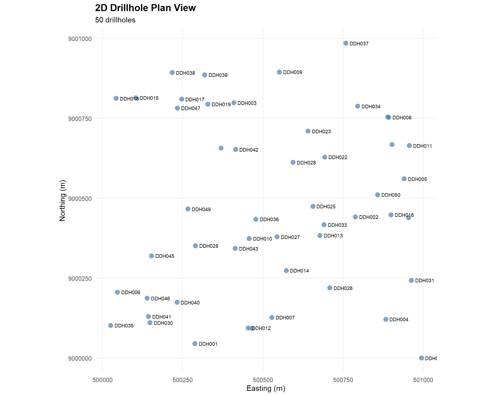
## 2D Drillhole Location Map
Let's start with a plan view showing collar locations.
### Basic Collar Map
```{r}
#| fig-width: 10
#| fig-height: 8
# Create 2D plan view
p_2d <- ggplot(collar_std, aes(x = x, y = y)) +
  geom_point(size = 3, alpha = 0.7, color = "steelblue") +
  geom_text(aes(label = hole_id),
            hjust = -0.2, vjust = 0.5,
            size = 2.5,
            check_overlap = TRUE) +
  coord_equal() +
  labs(
    title = "2D Drillhole Plan View",
    subtitle = paste(nrow(collar_std), "drillholes"),
    x = "Easting (m)",
    y = "Northing (m)"
  ) +
  theme_minimal() +
  theme(
    plot.title = element_text(size = 14, face = "bold"),
    panel.grid.minor = element_blank()
  )

p_2d
```
::: {.callout-note}
## Spatial Pattern Observations
Look for:
- **Clustering**: Groups of closely spaced holes
- **Gaps**: Areas with no drilling
- **Grid pattern**: Regular vs irregular spacing
- **Directional bias**: Preferential drilling directions
:::
### Interactive 2D Map with Average Grades
```{r}
#| fig-width: 10
#| fig-height: 8
# Calculate average grade per hole (example: using au_ppm)
avg_grades <- combined_data %>%
  group_by(hole_id, x, y) %>%
  summarise(
    avg_au = mean(au_ppm, na.rm = TRUE),
    max_au = max(au_ppm, na.rm = TRUE),
    .groups = 'drop'
  ) %>%
  filter(!is.na(avg_au))

# Create interactive plotly map
plot_ly(data = avg_grades,
        x = ~x, y = ~y,
        type = 'scatter', mode = 'markers',
        marker = list(
          size = 10,
          color = ~avg_au,
          colorscale = 'Viridis',
          showscale = TRUE,
          colorbar = list(title = "Avg Au<br>(ppm)")
        ),
        text = ~paste0(
          "Hole: ", hole_id, "<br>",
          "Avg Au: ", round(avg_au, 3), " ppm<br>",
          "Max Au: ", round(max_au, 3), " ppm"
        ),
        hoverinfo = 'text') %>%
  layout(
    title = "2D Drillhole Map: Average Gold Grades",
    xaxis = list(title = "Easting (m)"),
    yaxis = list(
      title = "Northing (m)",
      scaleanchor = "x",
      scaleratio = 1
    )
  )
```
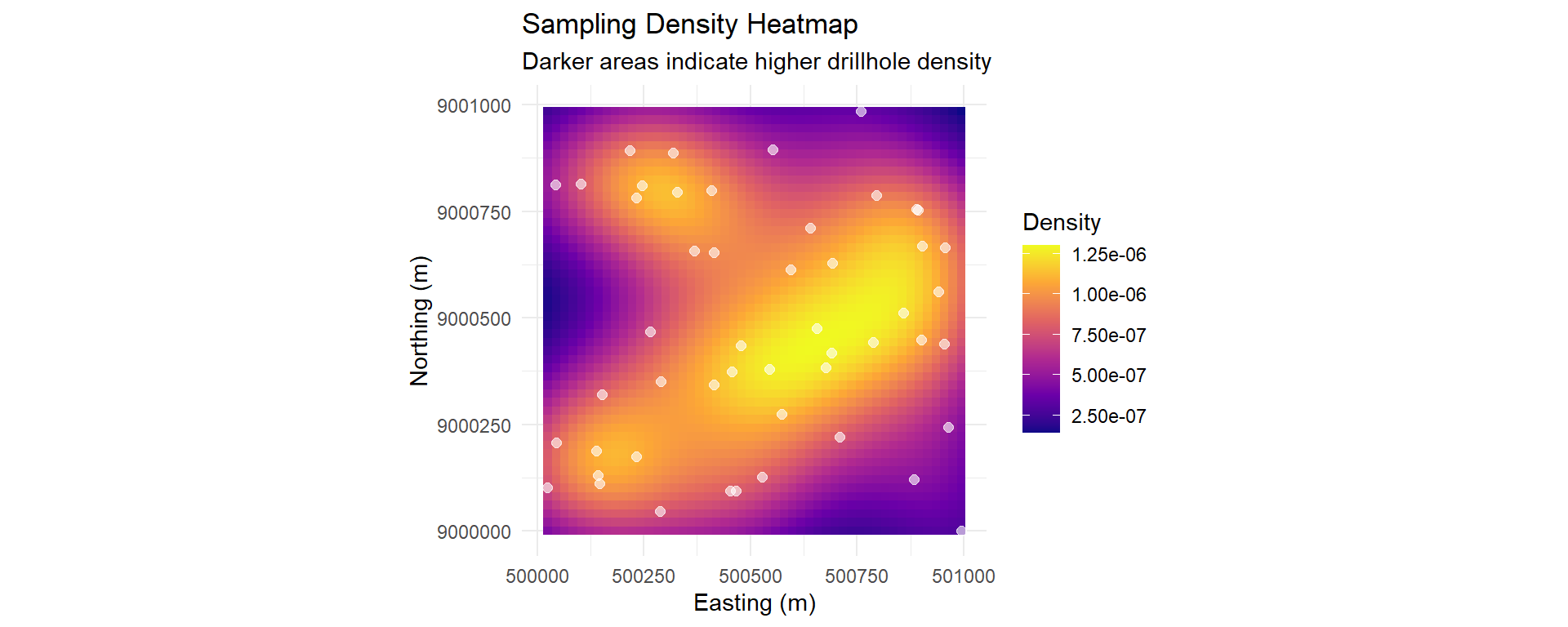
### Sampling Density Analysis
```{r}
#| fig-width: 10
#| fig-height: 4
# Calculate local sampling density
density_estimate <- MASS::kde2d(
  collar_std$x,
  collar_std$y,
  n = 50
)

# Convert to data frame for ggplot
density_df <- expand.grid(
  x = density_estimate$x,
  y = density_estimate$y
) %>%
  mutate(density = as.vector(density_estimate$z))

p_density <- ggplot() +
  geom_tile(data = density_df, aes(x = x, y = y, fill = density)) +
  scale_fill_viridis_c(option = "plasma", name = "Density") +
  geom_point(data = collar_std, aes(x = x, y = y),
             size = 2, color = "white", alpha = 0.6) +
  coord_equal() +
  labs(
    title = "Sampling Density Heatmap",
    subtitle = "Darker areas indicate higher drillhole density",
    x = "Easting (m)",
    y = "Northing (m)"
  ) +
  theme_minimal()

p_density
```
::: {.callout-important}
## Classification Implications
Sampling density directly impacts resource classification:
- **Dense areas**: Higher confidence → Measured/Indicated
- **Sparse areas**: Lower confidence → Indicated/Inferred
- **No data areas**: Extrapolation risk
:::
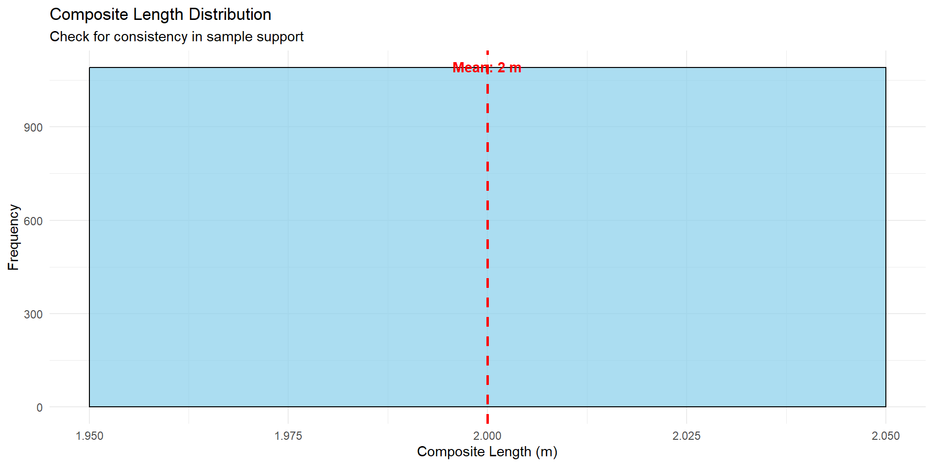
## Composite Length Analysis
Understanding sample support is critical for geostatistics.
```{r}
#| fig-width: 10
#| fig-height: 5
# Calculate composite lengths
combined_data <- combined_data %>%
  mutate(composite_length = to - from)

# Summary statistics
length_summary <- combined_data %>%
  summarise(
    `Min Length` = min(composite_length, na.rm = TRUE),
    `Q1` = quantile(composite_length, 0.25, na.rm = TRUE),
    `Median` = median(composite_length, na.rm = TRUE),
    `Mean` = mean(composite_length, na.rm = TRUE),
    `Q3` = quantile(composite_length, 0.75, na.rm = TRUE),
    `Max Length` = max(composite_length, na.rm = TRUE),
    `Std Dev` = sd(composite_length, na.rm = TRUE)
  )

datatable(length_summary,
          caption = "Table 1: Composite Length Statistics (meters)",
          options = list(dom = 't')) %>%
  formatRound(columns = 1:7, digits = 2)
# Histogram
p_length <- ggplot(combined_data, aes(x = composite_length)) +
  geom_histogram(bins = 30, fill = "skyblue", color = "black", alpha = 0.7) +
  geom_vline(xintercept = mean(combined_data$composite_length, na.rm = TRUE),
             color = "red", linetype = "dashed", size = 1) +
  annotate("text",
           x = mean(combined_data$composite_length, na.rm = TRUE),
           y = Inf,
           label = paste("Mean:", round(mean(combined_data$composite_length, na.rm = TRUE), 2), "m"),
           vjust = 2, color = "red", fontface = "bold") +
  labs(
    title = "Composite Length Distribution",
    subtitle = "Check for consistency in sample support",
    x = "Composite Length (m)",
    y = "Frequency"
  ) +
  theme_minimal()
p_length
```
::: {.callout-warning}
## Variable Sample Support Issues
Inconsistent sample lengths can cause:
- **Support effect**: Grade variance differences
- **Bias in estimation**: Longer samples overweighted
- **Variogram artifacts**: False spatial continuity
**Solution**: Composite to a consistent length (typically 1m or 2m)
:::
## 3D Visualization
Understanding the vertical distribution of data is essential.
```{r}
#| fig-width: 10
#| fig-height: 8
# Prepare 3D data with depth
data_3d <- combined_data %>%
  mutate(z_sample = z - ((from + to) / 2)) %>%
  filter(!is.na(x) & !is.na(y) & !is.na(z_sample) & !is.na(au_ppm))

# Sample data for performance (use 50% of data)
set.seed(123)
data_3d_sample <- sample_frac(data_3d, 0.5)

# Create 3D scatter plot
plot_ly(
  data = data_3d_sample,
  x = ~x, y = ~y, z = ~z_sample,
  type = 'scatter3d', mode = 'markers',
  marker = list(
    color = ~au_ppm,
    colorscale = 'Viridis',
    colorbar = list(title = "Au (ppm)"),
    size = 3
  ),
  text = ~paste0(
    "Hole: ", hole_id, "<br>",
    "Depth: ", round(from, 1), "-", round(to, 1), "m<br>",
    "Au: ", round(au_ppm, 3), " ppm"
  ),
  hoverinfo = 'text'
) %>%
  layout(
    title = "3D Drillhole Assay View",
    scene = list(
      xaxis = list(title = "Easting"),
      yaxis = list(title = "Northing"),
      zaxis = list(title = "Elevation (RL)", autorange = "reversed"),
      aspectratio = list(x = 1, y = 1, z = 0.5)
    )
  )
```
::: {.callout-tip}
## 3D Visualization Benefits
3D views help identify:
- Vertical trends in mineralization
- Dip and plunge of ore bodies
- Drilling depth coverage
- Spatial clustering in 3D space
:::
---
# PILLAR 3: Statistical Characterization
## Objective
Understand the **"personality"** of your grade data:
- What does the distribution look like?
- Are there outliers?
- Single or multiple populations?
- What top-cut value is appropriate?
## Univariate Statistics
### Summary Statistics by Grade Variable
```{r}
# Select numeric grade columns
grade_cols <- c("au_ppm", "ag_ppm", "cu_pct")

# Calculate comprehensive statistics
stats_summary <- combined_data %>%
  select(all_of(grade_cols)) %>%
  pivot_longer(everything(), names_to = "Grade", values_to = "Value") %>%
  group_by(Grade) %>%
  summarise(
    Count = sum(!is.na(Value)),
    Mean = mean(Value, na.rm = TRUE),
    Median = median(Value, na.rm = TRUE),
    `Std Dev` = sd(Value, na.rm = TRUE),
    CV = sd(Value, na.rm = TRUE) / mean(Value, na.rm = TRUE),
    Min = min(Value, na.rm = TRUE),
    Q1 = quantile(Value, 0.25, na.rm = TRUE),
    Q3 = quantile(Value, 0.75, na.rm = TRUE),
    Max = max(Value, na.rm = TRUE),
    Skewness = e1071::skewness(Value, na.rm = TRUE)
  ) %>%
  mutate(across(where(is.numeric), ~round(.x, 3)))

datatable(stats_summary,
          caption = "Table 2: Comprehensive Grade Statistics",
          options = list(scrollX = TRUE, pageLength = 10))
```
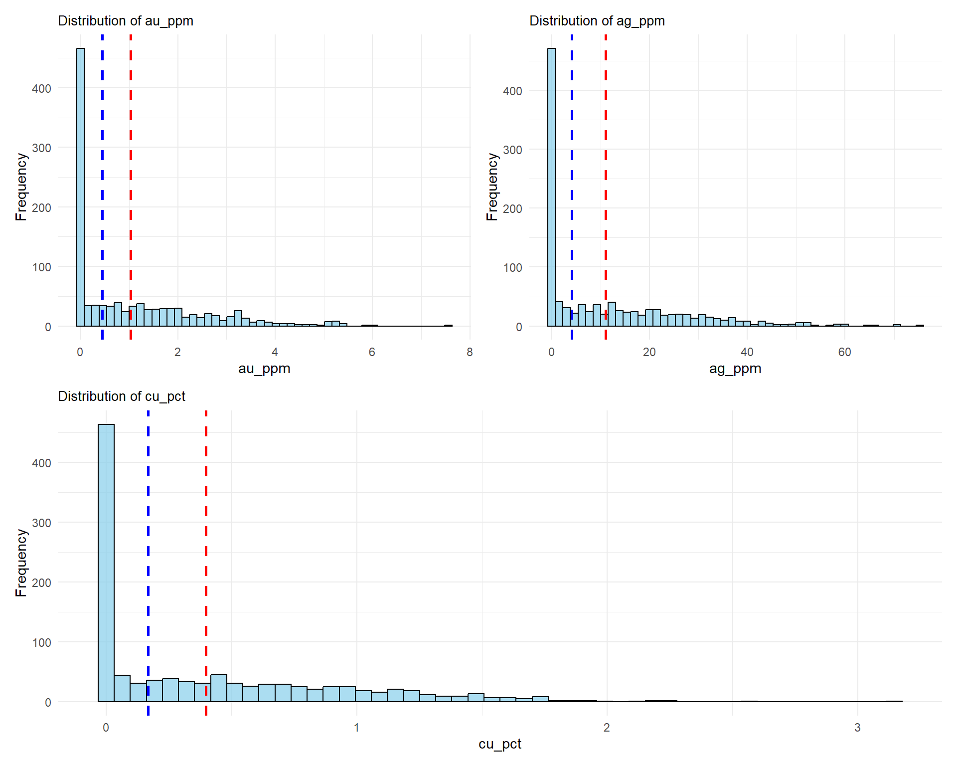
::: {.callout-note}
## Key Statistical Indicators
- **CV (Coefficient of Variation)**: Measure of variability (CV > 1 indicates high variability)
- **Skewness**: Positive skew common in grade data (long right tail)
- **Mean vs Median**: Large differences suggest outliers
:::
## Grade Distribution Analysis
### Histograms
```{r}
#| fig-width: 10
#| fig-height: 8
# Create histograms for each grade
plot_list <- lapply(grade_cols, function(col) {
  ggplot(combined_data, aes(x = .data[[col]])) +
    geom_histogram(bins = 50, fill = "skyblue", color = "black", alpha = 0.7) +
    geom_vline(xintercept = mean(combined_data[[col]], na.rm = TRUE),
               color = "red", linetype = "dashed", size = 1) +
    geom_vline(xintercept = median(combined_data[[col]], na.rm = TRUE),
               color = "blue", linetype = "dashed", size = 1) +
    labs(
      title = paste("Distribution of", col),
      x = col,
      y = "Frequency"
    ) +
    theme_minimal() +
    theme(plot.title = element_text(size = 10))
})

# Combine plots
(plot_list[[1]] | plot_list[[2]]) / plot_list[[3]]
```
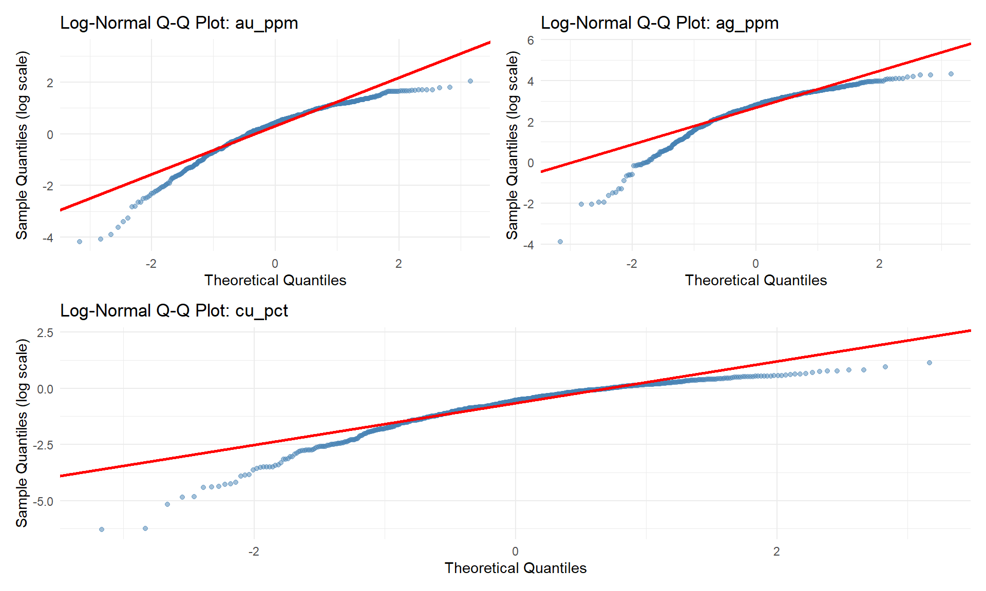
### Log-Normal Probability Plots
Essential for identifying populations and assessing normality.
```{r}
#| fig-width: 10
#| fig-height: 6
# Create Q-Q plots for log-transformed data
qq_plots <- lapply(grade_cols, function(col) {
  data_subset <- combined_data %>%
    filter(!is.na(.data[[col]]) & .data[[col]] > 0)

  ggplot(data_subset, aes(sample = log(.data[[col]]))) +
    stat_qq(color = "steelblue", alpha = 0.5) +
    stat_qq_line(color = "red", size = 1) +
    labs(
      title = paste("Log-Normal Q-Q Plot:", col),
      x = "Theoretical Quantiles",
      y = "Sample Quantiles (log scale)"
    ) +
    theme_minimal()
})

(qq_plots[[1]] | qq_plots[[2]]) / qq_plots[[3]]
```
::: {.callout-important}
## Population Identification
Breaks or changes in slope on Q-Q plots indicate:
- **Multiple populations**: Different geological/mineralization domains
- **Outliers**: High-grade samples requiring investigation
- **Mixed distributions**: Need for domain separation
**Action**: Use this information for domaining decisions!
:::
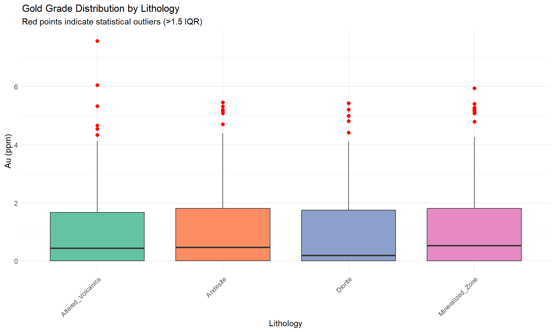
## Outlier Detection and Analysis
### Boxplots by Lithology
```{r}
#| fig-width: 10
#| fig-height: 6
# Focus on Au for outlier analysis
p_box <- ggplot(combined_data, aes(x = lithology, y = au_ppm, fill = lithology)) +
  geom_boxplot(outlier.colour = "red", outlier.shape = 16, outlier.size = 2) +
  scale_fill_brewer(palette = "Set2") +
  labs(
    title = "Gold Grade Distribution by Lithology",
    subtitle = "Red points indicate statistical outliers (>1.5 IQR)",
    x = "Lithology",
    y = "Au (ppm)"
  ) +
  theme_minimal() +
  theme(
    axis.text.x = element_text(angle = 45, hjust = 1),
    legend.position = "none"
  )

p_box
```
### Outlier Table
```{r}
# Calculate IQR-based outliers
outlier_threshold <- combined_data %>%
  summarise(
    Q1 = quantile(au_ppm, 0.25, na.rm = TRUE),
    Q3 = quantile(au_ppm, 0.75, na.rm = TRUE)
  ) %>%
  mutate(
    IQR = Q3 - Q1,
    lower_bound = Q1 - 1.5 * IQR,
    upper_bound = Q3 + 1.5 * IQR
  )

outliers <- combined_data %>%
  filter(au_ppm > outlier_threshold$upper_bound |
         au_ppm < outlier_threshold$lower_bound) %>%
  select(hole_id, from, to, lithology, au_ppm) %>%
  arrange(desc(au_ppm))

datatable(outliers,
          caption = paste("Table 3: Outlier Samples (n =", nrow(outliers), ")"),
          options = list(pageLength = 10, scrollX = TRUE)) %>%
  formatStyle('au_ppm', backgroundColor = '#ffebee', fontWeight = 'bold')
```
::: {.callout-warning}
## Outlier Treatment Options
1. **Keep as-is**: If geologically justified
2. **Top-cut (cap)**: Limit maximum grade
3. **Remove**: If analytical errors suspected
4. **Investigate**: Check for sample preparation issues
**Never** remove outliers without geological justification!
:::
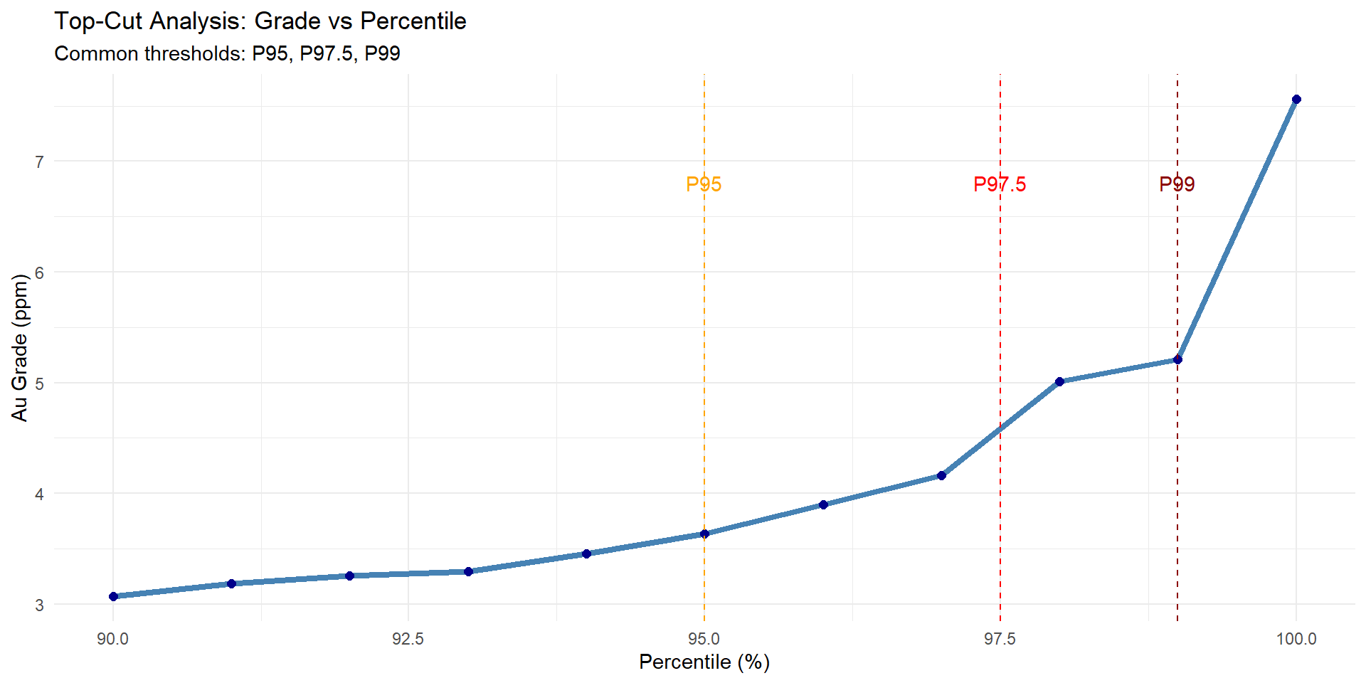
## Top-Cut Analysis
Determining appropriate grade capping values.
```{r}
#| fig-width: 10
#| fig-height: 5
# Calculate percentiles
percentiles <- seq(0.9, 1.0, by = 0.01)
percentile_values <- quantile(combined_data$au_ppm, probs = percentiles, na.rm = TRUE)

percentile_df <- data.frame(
  Percentile = percentiles * 100,
  Grade = percentile_values
)

# Plot grade vs percentile
p_percentile <- ggplot(percentile_df, aes(x = Percentile, y = Grade)) +
  geom_line(color = "steelblue", size = 1.5) +
  geom_point(size = 2, color = "darkblue") +
  geom_vline(xintercept = c(95, 97.5, 99),
             linetype = "dashed",
             color = c("orange", "red", "darkred")) +
  annotate("text", x = 95, y = max(percentile_values) * 0.9,
           label = "P95", color = "orange") +
  annotate("text", x = 97.5, y = max(percentile_values) * 0.9,
           label = "P97.5", color = "red") +
  annotate("text", x = 99, y = max(percentile_values) * 0.9,
           label = "P99", color = "darkred") +
  labs(
    title = "Top-Cut Analysis: Grade vs Percentile",
    subtitle = "Common thresholds: P95, P97.5, P99",
    x = "Percentile (%)",
    y = "Au Grade (ppm)"
  ) +
  theme_minimal()

p_percentile
```
### Impact of Top-Cutting
```{r}
# Compare statistics with different top-cuts
top_cuts <- c(Inf,
              quantile(combined_data$au_ppm, 0.95, na.rm = TRUE),
              quantile(combined_data$au_ppm, 0.975, na.rm = TRUE),
              quantile(combined_data$au_ppm, 0.99, na.rm = TRUE))

impact_df <- data.frame(
  Scenario = c("No Top-Cut", "P95 Cut", "P97.5 Cut", "P99 Cut"),
  `Cut Value` = round(top_cuts, 2),
  Mean = sapply(top_cuts, function(tc) {
    mean(pmin(combined_data$au_ppm, tc), na.rm = TRUE)
  }),
  Median = sapply(top_cuts, function(tc) {
    median(pmin(combined_data$au_ppm, tc), na.rm = TRUE)
  }),
  `Std Dev` = sapply(top_cuts, function(tc) {
    sd(pmin(combined_data$au_ppm, tc), na.rm = TRUE)
  }),
  CV = sapply(top_cuts, function(tc) {
    sd(pmin(combined_data$au_ppm, tc), na.rm = TRUE) /
      mean(pmin(combined_data$au_ppm, tc), na.rm = TRUE)
  })
) %>%
  mutate(across(where(is.numeric), ~round(.x, 3)))

datatable(impact_df,
          caption = "Table 4: Impact of Top-Cutting on Statistics",
          options = list(dom = 't'))
```
::: {.callout-tip}
## Selecting Top-Cut Values
Consider:
1. **Statistical analysis**: Probability plots, percentiles
2. **Geological context**: Are high grades real or analytical errors?
3. **Impact on resources**: Balance between grade and tonnage
4. **Industry standards**: P95-P99 common for precious metals
5. **Domaining**: Different top-cuts for different domains
**Document your decision** with geological and statistical justification!
:::
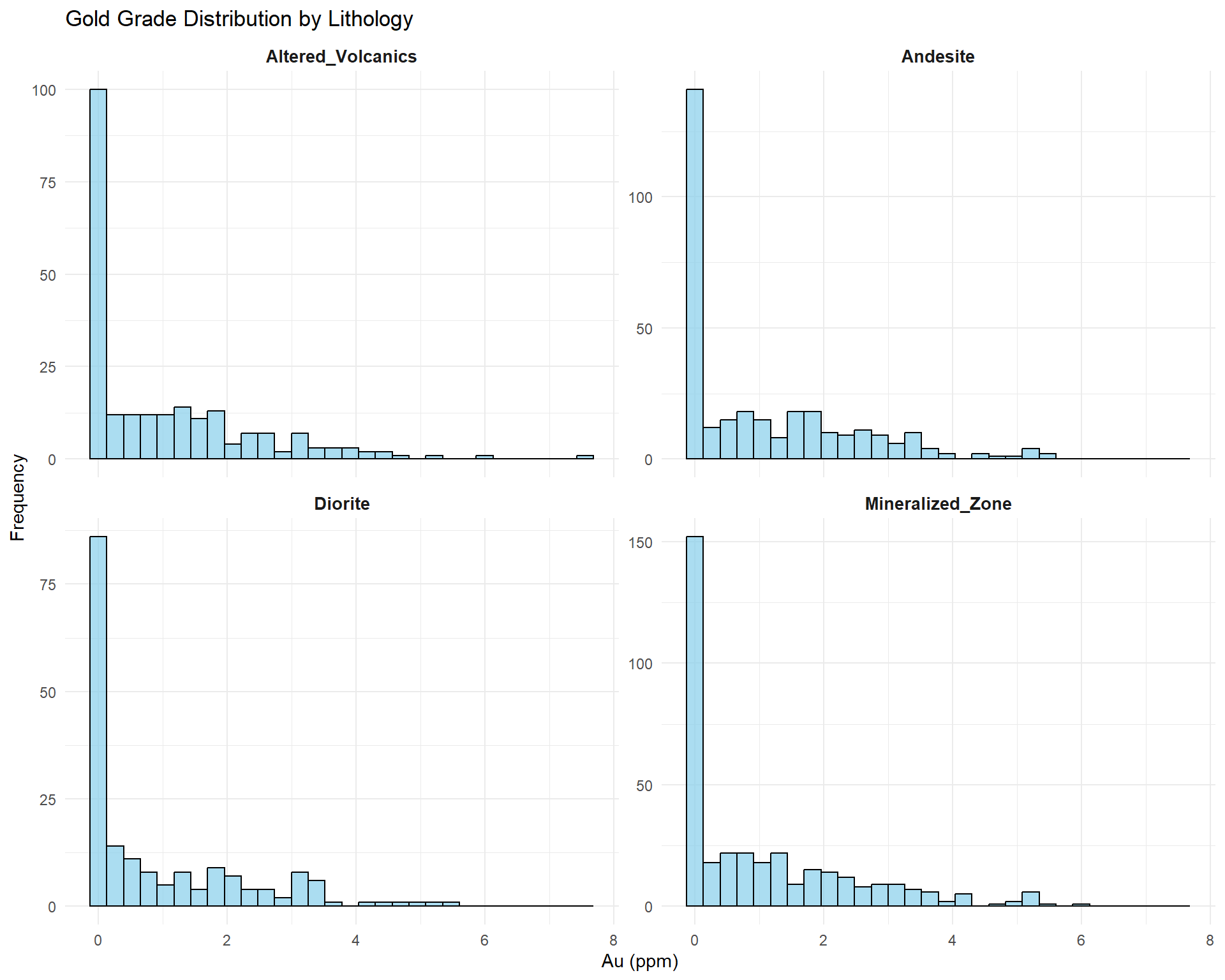
## Grade Distribution by Lithology
Understanding how grades vary by rock type.
```{r}
#| fig-width: 10
#| fig-height: 8
# Faceted histograms by lithology
ggplot(combined_data, aes(x = au_ppm)) +
  geom_histogram(bins = 30, fill = "skyblue", color = "black", alpha = 0.7) +
  facet_wrap(~ lithology, scales = "free_y", ncol = 2) +
  labs(
    title = "Gold Grade Distribution by Lithology",
    x = "Au (ppm)",
    y = "Frequency"
  ) +
  theme_minimal() +
  theme(strip.text = element_text(face = "bold", size = 10))
```
### Statistical Comparison by Lithology
```{r}
litho_stats <- combined_data %>%
  group_by(lithology) %>%
  summarise(
    Count = n(),
    Mean = mean(au_ppm, na.rm = TRUE),
    Median = median(au_ppm, na.rm = TRUE),
    `Std Dev` = sd(au_ppm, na.rm = TRUE),
    CV = sd(au_ppm, na.rm = TRUE) / mean(au_ppm, na.rm = TRUE),
    Max = max(au_ppm, na.rm = TRUE)
  ) %>%
  arrange(desc(Mean)) %>%
  mutate(across(where(is.numeric) & !Count, ~round(.x, 3)))

datatable(litho_stats,
          caption = "Table 5: Grade Statistics by Lithology",
          options = list(pageLength = 10)) %>%
  formatStyle(
    'Mean',
    background = styleColorBar(litho_stats$Mean, 'lightblue'),
    backgroundSize = '100% 90%',
    backgroundRepeat = 'no-repeat',
    backgroundPosition = 'center'
  )
```
::: {.callout-note}
## Geological Insights
This analysis reveals:
- **Host rocks**: Which lithologies contain mineralization?
- **Barren zones**: Low-grade lithologies to exclude?
- **Grade differences**: Justification for separate domains?
- **Continuity**: Are grades consistent within lithology?
:::
## Summary: Pillars 2 & 3
### Key Achievements
**Spatial Analysis (Pillar 2):**
✓ Visualized drillhole distribution in 2D and 3D
✓ Identified sampling density patterns
✓ Analyzed composite length consistency
✓ Recognized spatial trends in mineralization
**Statistical Analysis (Pillar 3):**
✓ Characterized grade distributions
✓ Identified outliers and proposed top-cuts
✓ Compared statistics by lithology
✓ Assessed data populations
### Checklist: Before Moving to Pillar 4
- [ ] Spatial patterns understood and documented
- [ ] Sampling density adequate for classification
- [ ] Grade populations identified
- [ ] Outliers investigated and treatment decided
- [ ] Top-cut values proposed with justification
- [ ] Lithology-grade relationships documented
::: {.callout-tip}
## Ready for Geological Controls?
With spatial and statistical understanding complete, you're ready to connect these patterns to geology in [Part 3: Geological Controls & Domain Definition](/posts/Geological Domain/).
:::
## Best Practices Recap
### Common Pitfalls to Avoid
1. **Ignoring spatial patterns** - Statistics alone aren't enough
2. **Over-relying on automation** - Always apply geological thinking
3. **Arbitrary top-cutting** - Document geological justification
4. **Skipping lithology analysis** - Rock types control grades
### Documentation Requirements
For JORC compliance, document:
- Spatial distribution maps and density analysis
- Statistical summary by domain/lithology
- Outlier treatment decisions with justification
- Top-cut analysis and selected values
- Population identification methodology
---
*Previous: [← Part 1 - Data Validation](/posts/Data Validation/)*
*Next: [Part 3 - Geological Controls & Domain Definition →](/posts/Geological Domain/)*